jjAnno 0.0.1
In fact, adding multiple different annotations (text, segment, rect, points, images and so on) beside the plot is needed. But we do not want to spend much time ,energy and code to render our raw figures. The Ai(Artificial Intelligence) is a good choice for you to produce a complex plot but without much accuracy.
Here I provide a package jjAnno that you can add different annotaions including point, text, rect, segemnt, image beside or inside the plot. This will be save your much time and cost to make a complex figure.
The following figures show the different annotations:

# install.packages("devtools")
devtools::install_github("junjunlab/jjAnno")

library(jjAnno)
note:
You should turn off the clip for your plot
coord_cartesian(clip = 'off')This function provides ArchR package's colors to plot.
Show all palettes:
# show all plattes
useMyCol(showAll = T)

# [1] "stallion"     "stallion2"    "calm"         "kelly"        "bear"         "ironMan"
# [7] "circus"       "paired"       "grove"        "summerNight"  "zissou"       "darjeeling"
# [13] "rushmore"     "captain"      "horizon"      "horizonExtra" "blueYellow"   "sambaNight"
# [19] "solarExtra"   "whitePurple"  "whiteBlue"    "comet"        "greenBlue"    "beach"
# [25] "coolwarm"     "fireworks"    "greyMagma"    "fireworks2"   "purpleOrange"
Draw these colors:
# plot colors
show_col(useMyCol('stallion',20))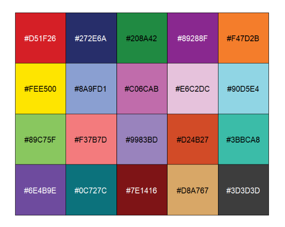
# ironMan
show_col(useMyCol('ironMan',15))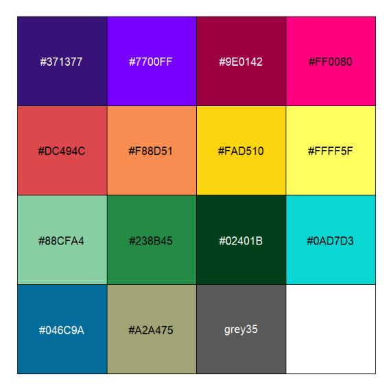
# whitePurple
show_col(useMyCol('whitePurple',9))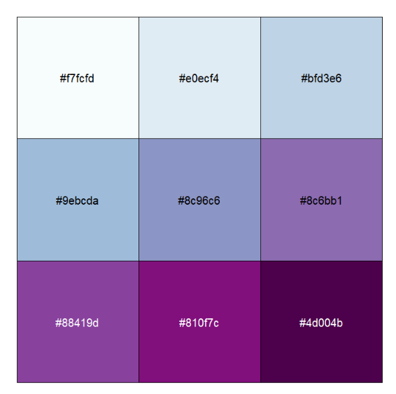
This function can be used to add some points annotations beside the plot or in plot.
Let's make a test data:
df <- data.frame(x = 1:10,y = sample(1:10,10),
                 x1 = LETTERS[1:10])
Make a simple plot:
library (ggplot2)

p <-
  ggplot(df, aes(x,x1)) +
  geom_point(aes(size = x,color = x,alpha = x)) +
  theme_bw(base_size = 14) +
  scale_x_continuous(breaks = seq(1,10,1)) +
  # scale_y_continuous(breaks = seq(1,10,1)) +
  scale_color_gradient(low = 'grey50',high = '#339933',name = '') +
  coord_cartesian(clip = 'off') +
  theme(aspect.ratio = 1,
        plot.margin = margin(t = 1,r = 1,b = 1,l = 1,unit = 'cm'),
        axis.text.x = element_text(vjust = unit(-1.5,'native')),
        legend.position = 'left') +
  xlab('') + ylab('')

p
Or we can use test data in this package:
data(p)Now we can use annoPoint to add points in our plot.
Default is the top position:
# default plot
annoPoint(object = p,
          annoPos = 'top',
          xPosition = c(1:10))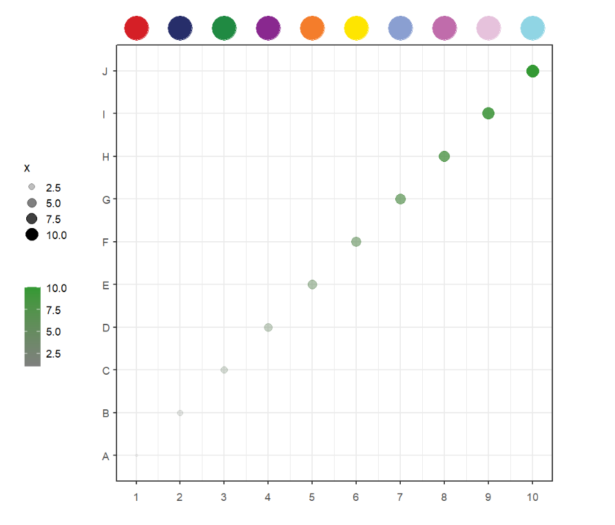
We can define multiple yPosition:
# specify yPosition
annoPoint(object = p,
          annoPos = 'top',
          xPosition = c(1:10),
          yPosition = rep(c(2,4,2,6,4),each = 2))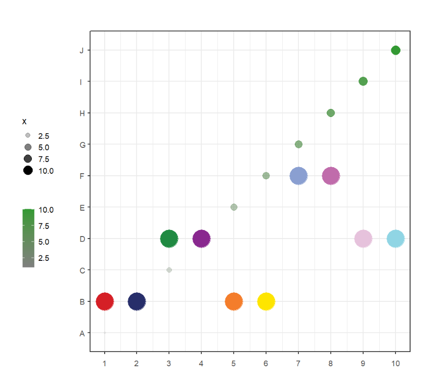
Add to right:
# add right
annoPoint(object = p,
          annoPos = 'right',
          yPosition = c(1:10))
Add to left:
# left
annoPoint(object = p,
          annoPos = 'left',
          yPosition = c(1:10))
We can supply xPosition to ajust a suitable position:
# supply xPosition to ajust
annoPoint(object = p,
          annoPos = 'right',
          yPosition = c(1:10),
          xPosition = 0.3)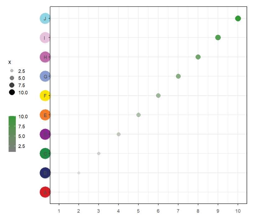
Change point size and shape:
# change point size and shape
annoPoint(object = p,
          annoPos = 'top',
          xPosition = c(1:10),
          ptSize = 2,
          ptShape = 25)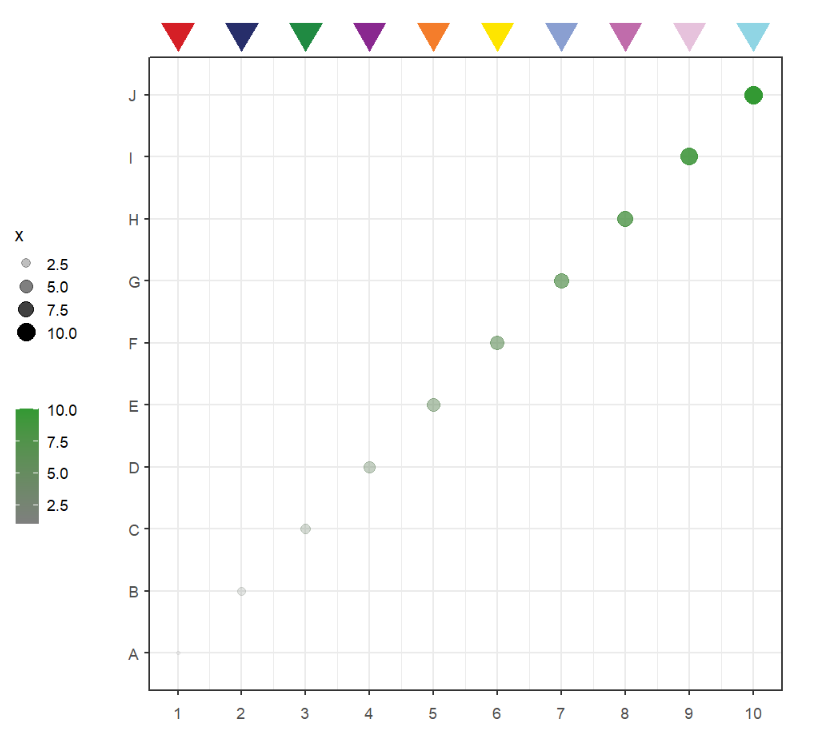
You can also add multiple annotations:
# add multiple annotations
p1 <- annoPoint(object = p,
                annoPos = 'top',
                xPosition = c(1:10),
                ptSize = 2,
                ptShape = 25)

annoPoint(object = p1,
          annoPos = 'right',
          yPosition = c(1:10),
          ptSize = 2,
          ptShape = 23)
This function can be used to add some rects annotations beside the plot or in plot.
Simple annotation:
# default plot
annoRect(object = p,
         annoPos = 'top',
         xPosition = c(1:10))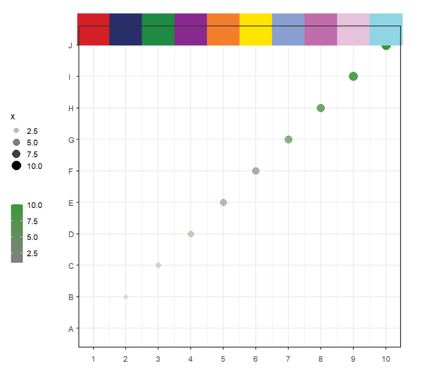
You can adjust the yPosition:
# adjust yPosition
annoRect(object = p,
         annoPos = 'top',
         xPosition = c(1:10),
         yPosition = c(11,11.5))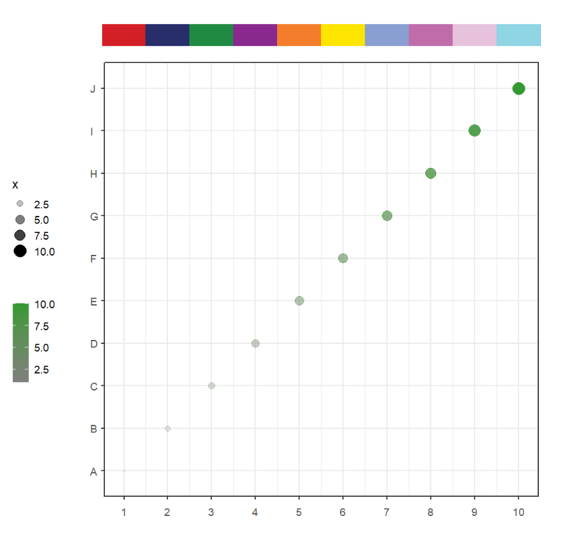
Change color alpha:
# change color alpha
annoRect(object = p,
         annoPos = 'top',
         xPosition = c(1:10),
         yPosition = c(11,11.5),
         alpha = 0.5)
Set rect width:
# adjust rectWidth
annoRect(object = p,
         annoPos = 'top',
         xPosition = c(1:10),
         yPosition = c(11,11.5),
         rectWidth = 0.9)
Change rect color and fill:
# change rect color and fill
annoRect(object = p,
         annoPos = 'top',
         xPosition = c(1:10),
         yPosition = c(11,11.5),
         rectWidth = 0.9,
         pCol = rep('black',10),
         pFill = rep('grey80',10))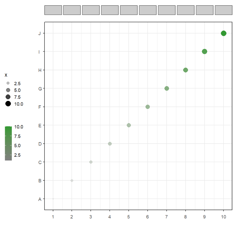
Change rect lty and lwd:
# change rect lty and lwd
annoRect(object = p,
         annoPos = 'top',
         xPosition = c(1:10),
         yPosition = c(11,11.5),
         rectWidth = 0.9,
         pCol = rep('black',10),
         pFill = rep('grey80',10),
         lty = 'dashed',
         lwd = 2)
Add only partial annotations:
# only add some annotations
annoRect(object = p,
         annoPos = 'top',
         xPosition = c(1,3,5,7,9),
         yPosition = c(11,11.5))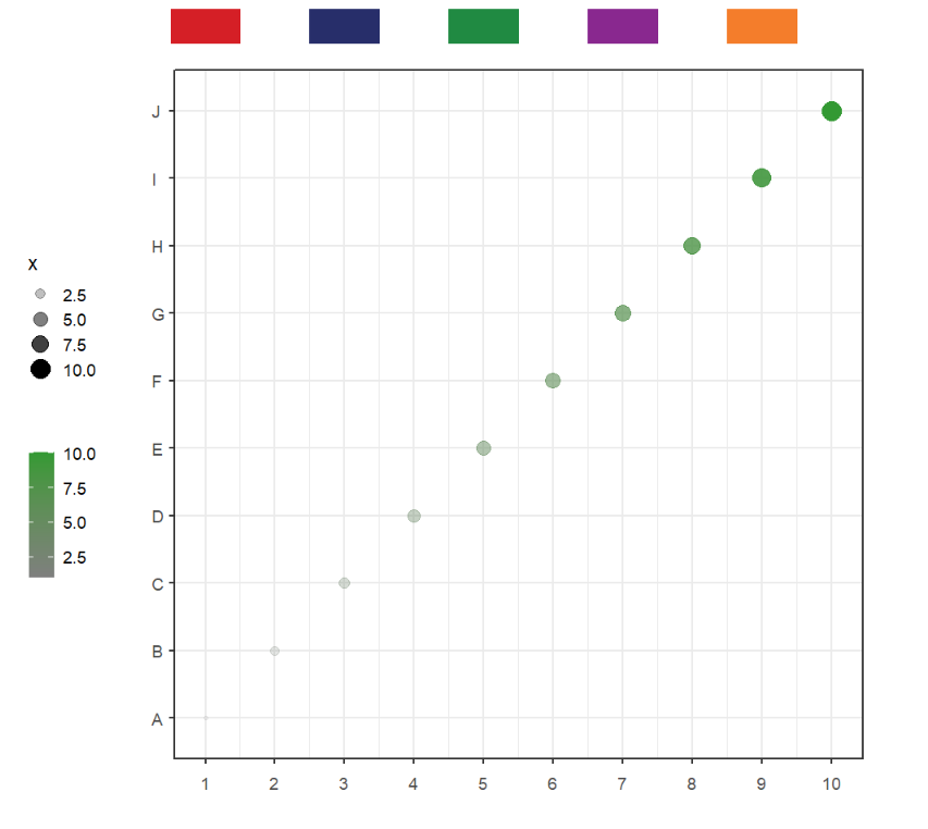
Supply your own coordinates to annotate:
# supply your own coordinates to annotate
annoRect(object = p,
         annoPos = 'top',
         annoManual = T,
         xPosition = list(c(1,6),
                          c(5,10)),
         yPosition = c(11,11.5),
         pCol = rep('black',2),
         lty = 'solid',
         lwd = 2)
You can supply multiple yPosition in list:
# multiple yPosition
annoRect(object = p,
         annoPos = 'top',
         annoManual = T,
         xPosition = list(c(1,6),
                          c(5,10)),
         yPosition = list(c(11,11.5),
                          c(11.5,12)),
         pCol = rep('black',2),
         lty = 'solid',
         lwd = 2)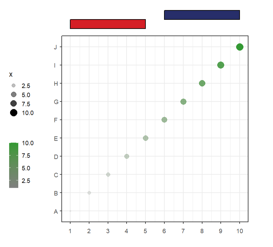
Add to right:
# add to right
annoRect(object = p,
         annoPos = 'right',
         yPosition = c(1:10),
         xPosition = c(10.5,11),
         rectWidth = 0.8)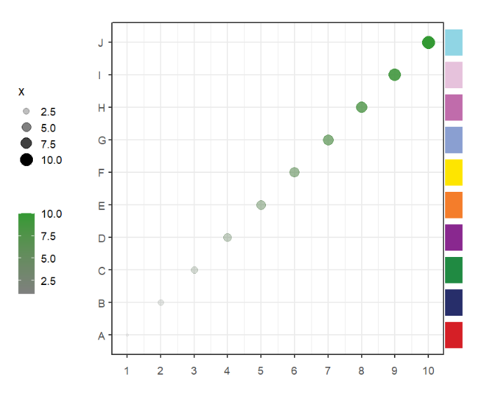
Add multiple annotations:
# add multiple
p1 <- annoRect(object = p,
               annoPos = 'top',
               xPosition = c(1:10),
               yPosition = c(11,11.5),
               rectWidth = 0.9,
               pCol = rep('black',10),
               pFill = rep('grey80',10),
               lty = 'dashed',
               lwd = 2)

# add second annotation
p2 <- annoRect(object = p1,
               annoPos = 'right',
               yPosition = c(1:10),
               xPosition = c(10.5,11),
               rectWidth = 0.8)

# add third annotation
annoRect(object = p2,
         annoPos = 'top',
         xPosition = c(1:10),
         yPosition = c(11.8,12.3),
         rectWidth = 0.8)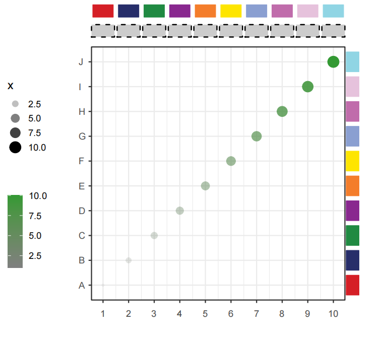
Load test data:
data(pgo)

pgo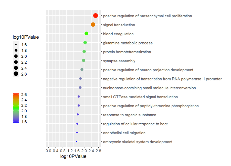
Here is the plot code:
# Plot
pgo <-
ggplot(df1,aes(x = log10PValue,y = Term)) +
  geom_point(aes(size = log10PValue,
                 color = log10PValue)) +
  scale_color_gradient2(low = 'blue',mid = 'green',high = 'red',
                        name = '',midpoint = 2.1) +
  scale_y_discrete(position = 'right') +
  scale_x_continuous(breaks = seq(0,2.8,0.4),limits = c(0,2.8)) +
  theme_grey(base_size = 14) +
  theme(legend.position = 'left',
        plot.margin = margin(t = 1,r = 1,b = 1,l = 1,unit = 'cm'),
        aspect.ratio = 2.5
        ) +
  coord_cartesian(clip = 'off') +
ylab('')Add 15 rects:
# another example annotation GO terms
annoRect(object = pgo,
         annoPos = 'right',
         yPosition = c(1:15),
         pCol = rep('transparent',15),
         pFill = rep(c('#F5F0BB','#C4DFAA','#90C8AC'),each = 5),
         xPosition = c(3,10),
         rectWidth = 1)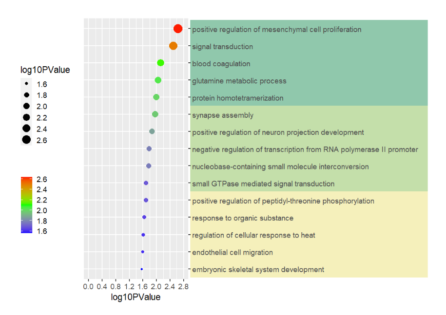
Supply own coordinates to add(3 rects):
# annotate mannually
annoRect(object = pgo,
         annoPos = 'right',
         annoManual = T,
         xPosition = c(3,10),
         yPosition = list(c(0.5,5.5,10.5),
                          c(5.5,10.5,15.5)),
         pCol = rep('black',3),
         pFill = c('#F5F0BB','#C4DFAA','#90C8AC'))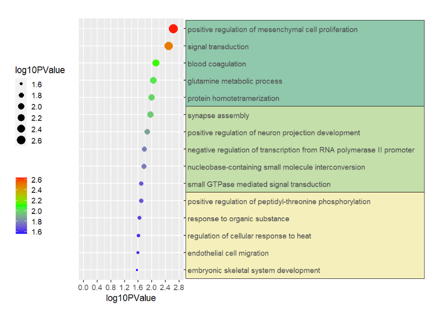
This function can be used to add some segments annotations beside the plot or in plot.
Simple annotation:
# default plot
annoSegment(object = p,
            annoPos = 'top',
            xPosition = c(1:10))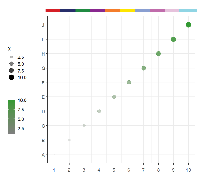
Adjust rectWidth:
# adjust rectWidth
annoSegment(object = p,
            annoPos = 'top',
            xPosition = c(1:10),
            segWidth = 0.8)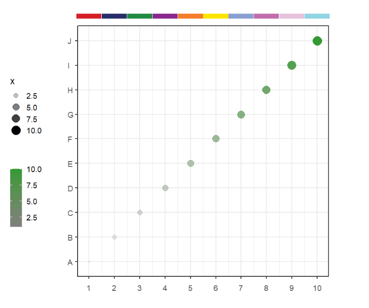
Add segments with arrow:
library(ggplot2)

# add segments with arrow
annoSegment(object = p,
            annoPos = 'top',
            xPosition = c(1:10),
            segWidth = 0.9,
            lwd = 1,
            mArrow = arrow(ends = 'both',
                           length = unit(0.2,'cm'),
                           type = 'closed'))
Change rect color and fill:
# change rect color and fill
annoSegment(object = p,
            annoPos = 'top',
            xPosition = c(1:10),
            segWidth = 0.8,
            pCol = useMyCol('horizon',10))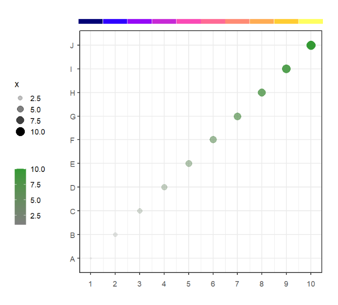
Add segments with branch:
# add branch
annoSegment(object = p,
            annoPos = 'top',
            xPosition = c(1:10),
            segWidth = 0.8,
            addBranch = T,
            lwd = 4)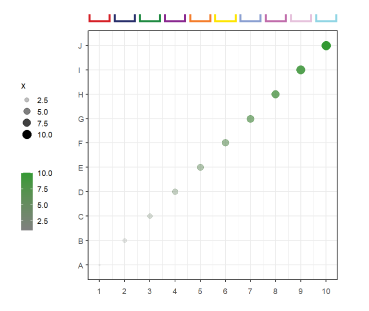
Change branch direction:
# change branch direction
annoSegment(object = p,
            annoPos = 'top',
            xPosition = c(1:10),
            segWidth = 0.8,
            addBranch = T,
            lwd = 4,
            branDirection = -1)
Add to botomn:
# add to botomn
annoSegment(object = p,
            annoPos = 'botomn',
            xPosition = c(1:10),
            segWidth = 0.8,
            addBranch = T,
            lwd = 4)
Add to right:
# add to right
annoSegment(object = p,
            annoPos = 'right',
            yPosition = c(1:10),
            segWidth = 0.8,
            addBranch = T,
            lwd = 4,
            branDirection = -1)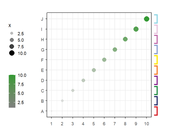
Add branch with arrow:
# add to botomn and make branch taged with arrow
annoSegment(object = p,
            annoPos = 'botomn',
            xPosition = c(1:10),
            segWidth = 0.8,
            addBranch = T,
            lwd = 3,
            bArrow = arrow(length = unit(0.2,'cm'),
                           ends = 'last'))
Add text label:
# add text label
annoSegment(object = p,
            annoPos = 'top',
            xPosition = c(1:10),
            segWidth = 0.8,
            addBranch = T,
            lwd = 4,
            branDirection = -1,
            addText = T,
            textLabel = paste0('anno',1:10,sep = ''),
            textRot = 0,
            textSize = 15)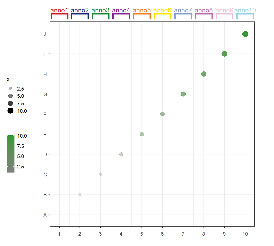
Add text space relative to segments:
# add text space from segments
annoSegment(object = p,
            annoPos = 'top',
            xPosition = c(1:10),
            segWidth = 0.8,
            addBranch = T,
            lwd = 4,
            branDirection = -1,
            addText = T,
            textLabel = paste0('anno',1:10,sep = ''),
            textRot = 45,
            textSize = 15,
            textHVjust = 0.5)
Change text color:
# change text color
annoSegment(object = p,
            annoPos = 'top',
            xPosition = c(1:10),
            segWidth = 0.8,
            addBranch = T,
            lwd = 4,
            branDirection = -1,
            addText = T,
            textLabel = paste0('anno',1:10,sep = ''),
            textRot = 45,
            textSize = 15,
            textHVjust = 0.5,
            textCol = rep('grey50',10))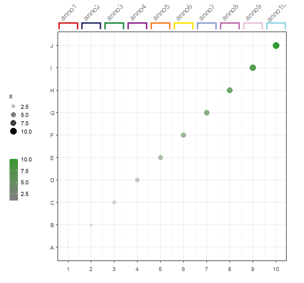
Change segments yPosition:
# change yPosition
annoSegment(object = p,
            annoPos = 'top',
            xPosition = c(1:10),
            segWidth = 0.8,
            pCol = useMyCol('horizon',10),
            yPosition = 5)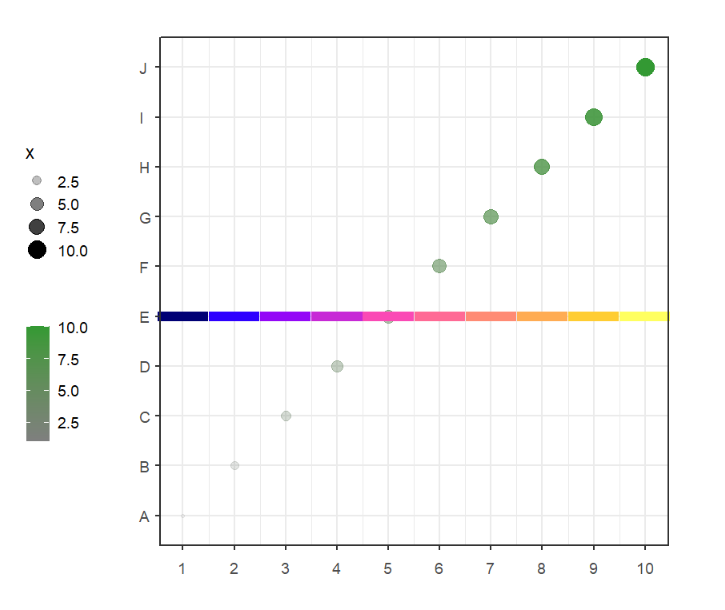
Supply your own coordinates to annotate:
# supply your own coordinates to annotate
annoSegment(object = p,
            annoPos = 'top',
            annoManual = T,
            xPosition = list(c(1,6),
                             c(5,10)),
            yPosition = 11,
            pCol = c('green','orange'))
Add branch to plot:
# add branch to plot
annoSegment(object = p,
            annoPos = 'top',
            annoManual = T,
            addBranch = T,
            lwd = 3,
            segWidth = 0.5,
            xPosition = list(c(1,6),
                             c(5,10)),
            yPosition = c(11,11),
            pCol = c('green','orange'),
            branDirection = -1)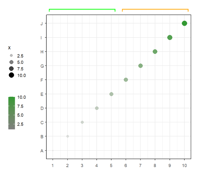
Add to right:
# add to right
annoSegment(object = p,
            annoPos = 'right',
            yPosition = c(1:10),
            segWidth = 0.8)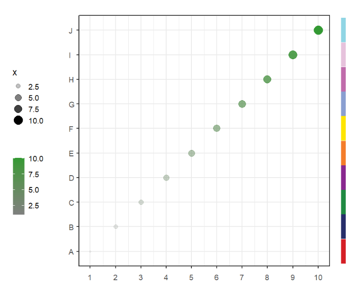
Annotate GO plot with segments:
# annotate mannually
annoSegment(object = pgo,
            annoPos = 'left',
            annoManual = T,
            xPosition = rep(-0.15,3),
            yPosition = list(c(1,6,11),
                             c(5,10,15)),
            pCol = c('#F5F0BB','#C4DFAA','#90C8AC'),
            segWidth = 1)
This function can be used to add some images annotations beside the plot or in plot.
Load images:
img1 <- system.file("extdata/animal-img/", "1.jpg", package = "jjAnno")
img2 <- system.file("extdata/animal-img/", "2.jpg", package = "jjAnno")
img3 <- system.file("extdata/animal-img/", "3.jpg", package = "jjAnno")
img4 <- system.file("extdata/animal-img/", "4.jpg", package = "jjAnno")
img5 <- system.file("extdata/animal-img/", "5.jpg", package = "jjAnno")
img6 <- system.file("extdata/animal-img/", "6.jpg", package = "jjAnno")
img7 <- system.file("extdata/animal-img/", "7.jpg", package = "jjAnno")
img8 <- system.file("extdata/animal-img/", "8.jpg", package = "jjAnno")
img9 <- system.file("extdata/animal-img/", "9.jpg", package = "jjAnno")
img10 <- system.file("extdata/animal-img/", "10.jpg", package = "jjAnno")

imgs <- c(img1,img2,img3,img4,img5,img6,img7,img8,img9,img10)
Simple annotation:
# add legend
annoImage(object = p,
          annoPos = 'top',
          xPosition = c(1:10),
          images = imgs,
          yPosition = c(11,12))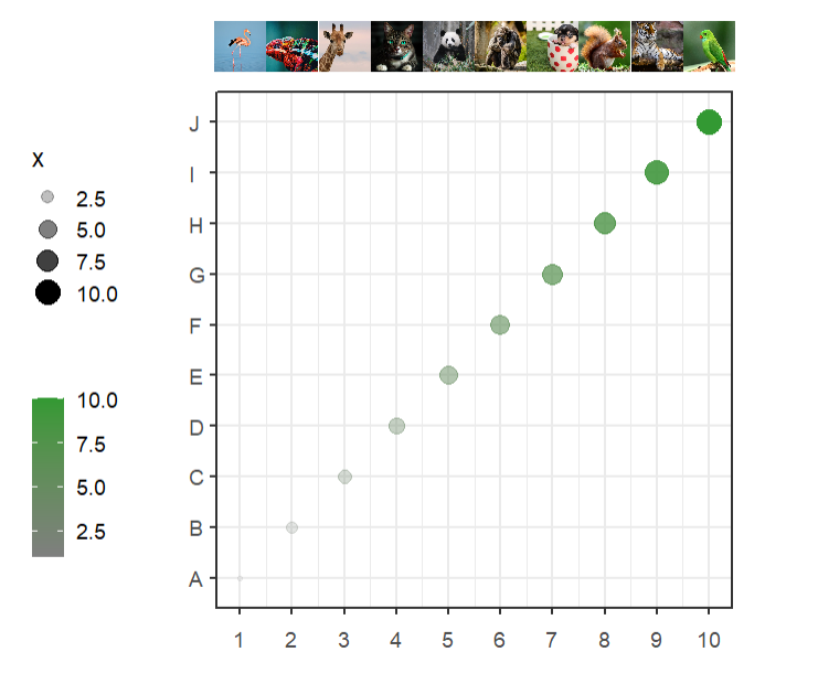
Ajust width:
# change width
annoImage(object = p,
          annoPos = 'top',
          xPosition = c(1:10),
          images = imgs,
          yPosition = c(11,11.8),
          segWidth = 0.8)
Add to right:
# add to right
annoImage(object = p,
          annoPos = 'right',
          yPosition = c(1:10),
          images = imgs,
          xPosition = c(11,11.8),
          segWidth = 0.8)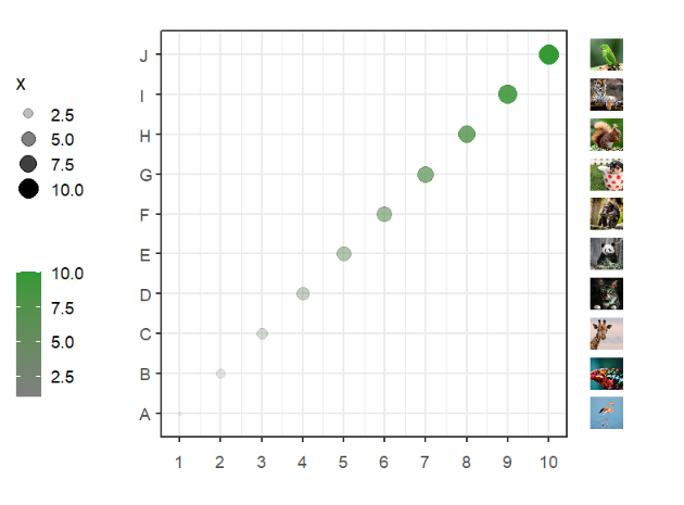
Add to botomn:
# add to botomn
annoImage(object = p,
          annoPos = 'botomn',
          xPosition = c(1:10),
          images = imgs,
          yPosition = c(-1.2,-0.4),
          segWidth = 0.8)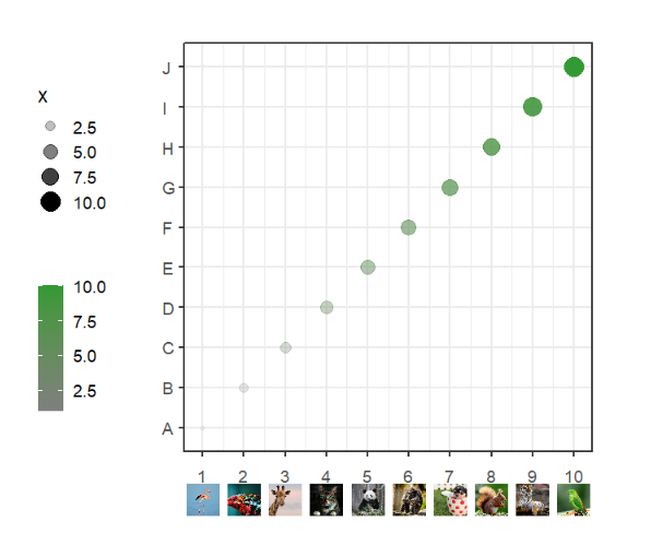
Annotate manually:
# annotate manually
annoImage(object = p,
          annoPos = 'right',
          yPosition = list(c(1:10),
                           c(1:10)),
          images = imgs,
          annoManual = T,
          xPosition = list(rep(c(11,11.8),each = 5),
                           rep(c(11.8,12.6),each = 5)),
          segWidth = 0.8)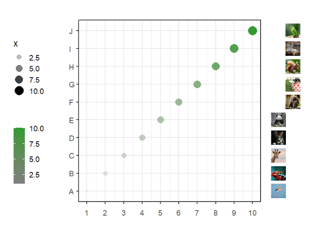
This function can be used to add some legend annotations beside the plot or in plot.
Simple annotation:
# add legend
annoLegend(object = p,
           labels = paste('legend ',1:5),
           pch = 21,
           col = 'black',
           fill = useMyCol('paired',5),
           textSize = 15)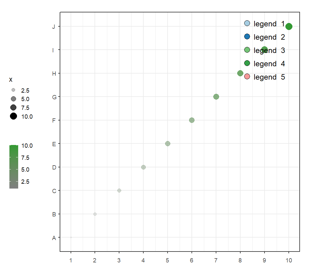
Change legend position:
# change pos
annoLegend(object = p,
           relPos = c(0.2,0.9),
           labels = paste('legend ',1:5),
           pch = 21,
           col = 'black',
           fill = useMyCol('paired',5),
           textSize = 15)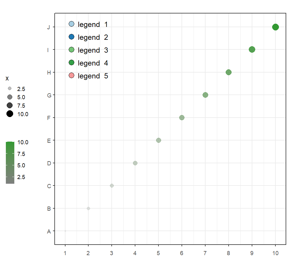
Add multiple shapes:
# multiple shapes
annoLegend(object = p,
           relPos = c(0.2,0.9),
           labels = paste('legend ',1:5),
           pch = 21:25,
           col = 'black',
           fill = useMyCol('paired',5),
           textSize = 15)
Define x and y position:
# define x and y position
annoLegend(object = p,
           xPosition = 12,
           yPosition = 5,
           labels = paste('legend ',1:5),
           pch = 21:25,
           col = 'black',
           fill = useMyCol('paired',5),
           textSize = 15)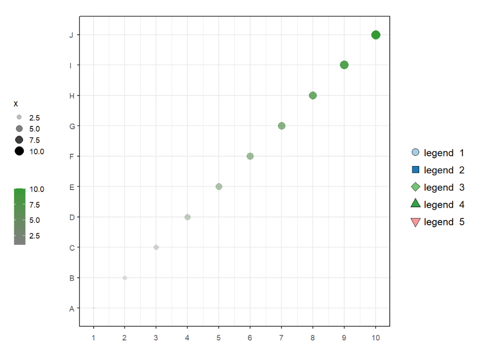
Let's see an example:
data("pdot")

pdot
We add some annotations on this figure:
# add segment
P1 <- annoSegment(object = pdot,
                  annoPos = 'top',
                  xPosition = c(1:21),
                  yPosition = 8.8,
                  segWidth = 0.7,
                  pCol = c(useMyCol('stallion',20),'orange'))

# add rect1
P2 <- annoRect(object = P1,
               annoPos = 'left',
               annoManual = T,
               yPosition = list(c(0.5,4.5),
                                c(4.5,8.5)),
               xPosition = c(-3.5,0.3),
               pCol = rep('white',2),
               pFill = useMyCol('calm',2),
               alpha = 0.5)

# add rect2
P3 <- annoRect(object = P2,
               annoPos = 'left',
               annoManual = T,
               yPosition = list(c(2.5),
                                c(6.5)),
               xPosition = c(-3.5,16.5),
               pCol = 'black',
               pFill = 'transparent',
               lty = 'dashed',
               lwd = 3)

# add branch
P4 <- annoSegment(object = P3,
                  annoPos = 'top',
                  annoManual = T,
                  xPosition = list(c(1,3,4,7,9,11,12,15,17,19,20),
                                   c(2,3,6,8,10,11,14,16,18,19,21)),
                  yPosition = 9.2,
                  segWidth = 0.8,
                  pCol = rep('black',11),
                  addBranch = T,
                  branDirection = -1,
                  lwd = 3)

# add text
text <- c('Mesothelial','Extragonadal','Gonadal','Supporting lineage','Interstitial lineage',
          'Testis fate','Early supporting','Granulosa','Sertoli','sPAX8','Mesenchymal')

# add text
annoSegment(object = P4,
            annoPos = 'top',
            annoManual = T,
            xPosition = list(c(1,3,4,7,9,11,12,15,17,19,20),
                             c(2,3,6,8,10,11,14,16,18,19,21)),
            yPosition = 9.2,
            segWidth = 0.8,
            pCol = rep('black',11),
            addBranch = T,
            branDirection = -1,
            lwd = 3,
            addText = T,
            textLabel = text,
            textCol = c(rep('black',5),'blue',rep('black',5)),
            textRot = 45,
            hjust = 0)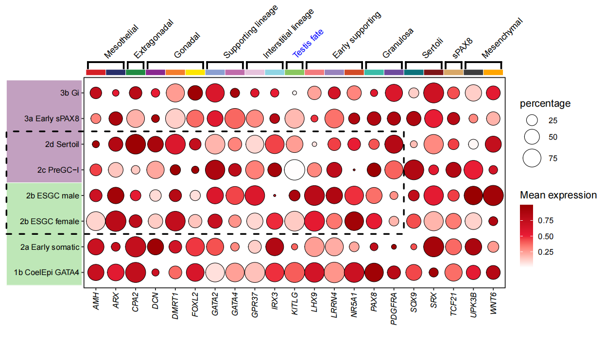
More paremeters see:
?useMyCol
?annoPoint
?annoRect
?annoSegment
?annoImage
?annoLegend