An implementation of an alternative embedding algorithm for graph data. Based on the paper Graph DNA: Deep Neighborhood Aware Graph Encoding for Collaborative Filtering (Liwei Wu et. al)
The goal of Graph DNA is to create a memory and time efficient way to embed graph data into a format that is more easily consumed by Graph Neural Networks, while still preserving as much structural insight as possible.
Existing methods localize vertices with message passing using adjacency matrix multiplication + loss function minimization, but have trouble gathering structural insight from graphs beyond 1-2 hops without pushing exponential time and space limits.
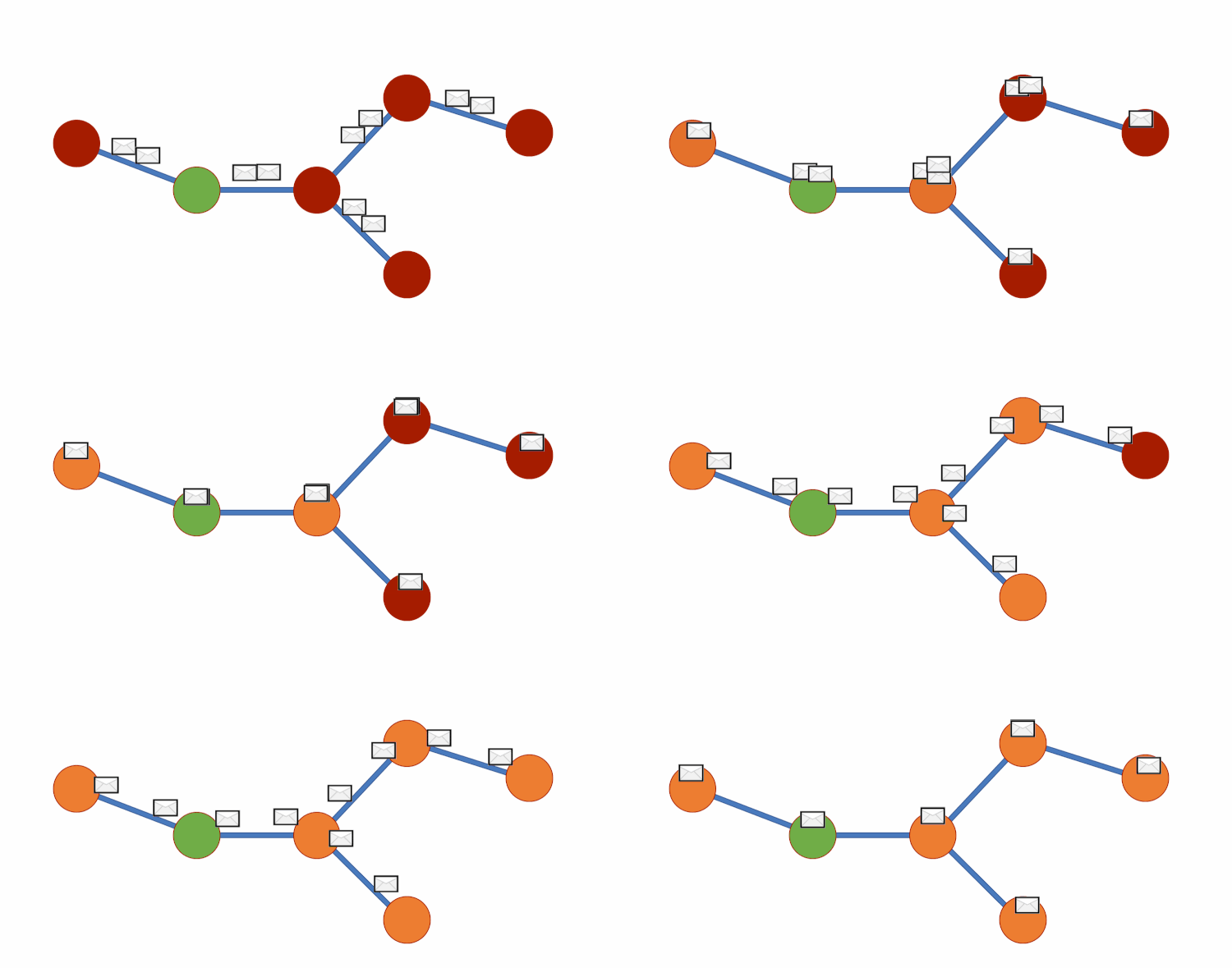
Graph DNA uses bloom filters and gossip algorithms to gain deeper neighbourhood insight at a much lower cost. The bloom filters let vertex embeddings inherently hold information about which other vertices influence them. We can then create a new bipartite graph G', where each vertex v of G is adjacent to a corresponding meta-vertex if and only if the corresponding bit in the Bloom filter for v has been activated. See diagram below for a visual representation. We can then perform standard filtering algorithms on G' to obtain deep neighbourhood aware feature aggregations at a fraction of the cost. Finally, for predictions to be made we disregard meta-vertices. Again, all theory is from this paper (Liwei Wu et. al).

(https://arxiv.org/pdf/1905.12217.pdf, Liwei Wu et. al)
Graph Convolutional Networks are extremely powerful tools in biology, social networks & eCommerce with applications including drug interaction prediction, and advanced reccomendation systems.
Demonstrating more time and memory efficient methods for creating graph embeddings is essential in pushing forward these advancments, and making graph data more easily consumed by neural networks.
As seen in examples.py we can recreate the graph on page 5, and generate its DNA encoding as follows:
figure_1 = Graph(5, [[0,1], [1,2], [2,3], [2,4]])

# generate dna encoding and display results for each vertex
dna_encoding = figure_1.generate_dna_encoding(depth=2, filter_capacity=3)
print(dna_encoding)

>>> [[1, 1, 1, 0, 0, 1, 1, 1, 1, 1, 0, 1, 1, 1, 0, 1],
     [1, 1, 1, 1, 0, 1, 1, 1, 1, 1, 1, 1, 1, 1, 0, 1],
     [1, 1, 1, 1, 0, 1, 1, 1, 1, 1, 1, 1, 1, 1, 0, 1],
     [1, 0, 1, 1, 0, 1, 1, 1, 1, 1, 1, 0, 1, 1, 0, 1],
     [1, 0, 1, 1, 0, 1, 1, 1, 1, 1, 1, 0, 1, 1, 0, 1]]

# construct our meta bipartite graph and display the set of edges
meta_graph = figure_1.generate_meta_graph(dna_encoding)
print(meta_graph.edges)
>>> [[0, 5], [0, 6], [0, 7], [0, 10], [0, 11], [0, 12], [0, 13], [0, 14], [0, 16], [0, 17], [0, 18], [0, 20],
    [1, 5], [1, 6], [1, 7], [1, 8], [1, 10], [1, 11], [1, 12], [1, 13], [1, 14], [1, 15], [1, 16], [1, 17], [1, 18], [1, 20],
    [2, 5], [2, 6], [2, 7], [2, 8], [2, 10], [2, 11], [2, 12], [2, 13], [2, 14], [2, 15], [2, 16], [2, 17], [2, 18], [2, 20],
    [3, 5], [3, 7], [3, 8], [3, 10], [3, 11], [3, 12], [3, 13], [3, 14], [3, 15], [3, 17], [3, 18], [3, 20],
    [4, 5], [4, 7], [4, 8], [4, 10], [4, 11], [4, 12], [4, 13], [4, 14], [4, 15], [4, 17], [4, 18], [4, 20]]
The output is the generated embedding for each vertex. We can see that vertices 3,4 and 1,2 respectively get the same embeddings with d=2 just as depicted in Figure 1 in the paper.
