Tim Menzies, Oussama Elrawas, Jairus Hihn, Martin Feather, Ray Madachy, and Barry Boehm. 2007. The business case for automated software engineering In Proceedings of the 22nd IEEE/ACM International Conference on Automated Software Engineering (ASE '07). Association for Computing Machinery, New York, NY, USA, 303–312.
- Lessons from this case study
- To handle uncertainty, simulate across the variability.
- Not all variables matter
- Useful to combine optimizers and data mining
- Simple often works well
- This is not how I would do this in 2023
(To avoid traps, before you sober up, get a little drunk and take some risks.)

def SIMULATED-ANNEALING(problem,schedule)
  returns: a solution state
  current ← problem.INITIAL-STATE
  for t = 1 to Tmax do
     T ← schedule(t)
 # e.g. T=t
     if T = 0 then return current

     next ← a randomly selected successor of current

     ΔE ← VALUE(next) - VALUE(current)

     if ΔE > 0 then current ← next

     else current ← next only with probability eΔE/T
return current(Why just mutate on example?)

def GENETIC-ALGORITHM(population, FITNESS-FN)
 returns: an individual

 inputs:  population, the initial random population of individuals
          FITNESS-FN, a function that measures the fitness of an individual
 repeat

    population ← [MUTATE(RECOMBINE(SELECT(2, population, FITNESS-FN)))

                 for i in population]

  until some individual is fit enough, or enough time has elapsed
  return the best individual in population, according to FITNESS-FN
def SELECT(ρ, population, FITNESS-FN)
returns: a set of ρ individuals
election ← a uniform random sample of 2 * ρ individuals from population
return the top ρ individuals in selection, ranked by FITNESS-FNdef RECOMBINE(x, y)
returns:an individual
inputs: x,y, parent individuals
n ← LENGTH(x)
crossover ← random integer from 0 to n
return APPEND(x[0:crossover], y[crossover: n])(Base mutation on an archive of successful candidates.)
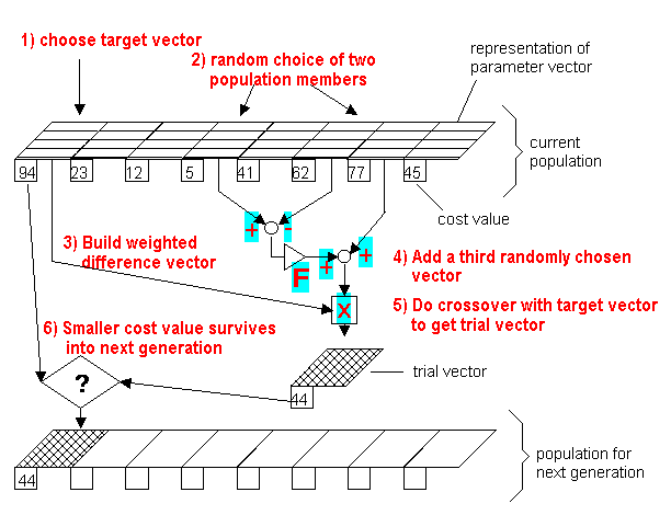
- Choose the parameters:
-
$\text{NP}$ = population size, i.e. the number of candidate agents or "parents"; for$n$ attributes, a typical setting is$10*n$ . -
$\text{CR} \in [0,1]$ = called the ''crossover probability'' -
$F \in [0,2]$ = ''differential weight''. - Typical settings are
$F = 0.8$ and$CR = 0.9$ .
-
- Create a population of
$\text{Pop}=\text{NP}$ individuals at random - Repeat until a termination criterion is met (e.g. number of iterations performed, or adequate fitness reached):
- For
${x}\in\text{Pop}$ :- Pick any
${a},{b},{c}\in\text{Pop}$ - Pick one attribute index
$R$ at random (good idea that at least one part of the old survives to new) $y= \text{copy}(x)$ - For each independent input attribute
$i \in {1,\ldots,n}$ - If
$\text{rand}(0,1)<\text{CR}$ or$i=R$ then$y_i = a_i + F \times (b_i-c_i)$
- If
- If
$y$ better than$x$ , replace${x}$ in$\text{Pop}$ with$y$
- Pick any
- For
- Pick the agent from the population that has the best fitness and return it as the best found candidate solution.
- When working with symbolic attributes
$y_i = a_i \vee ((\text{rand}()<\text{CR}) \wedge b_i \vee c_i)$
- Traditional DE uses bdom which means often many new things
$x$ seem to be the same as old things$y$ - ye olde DE would add such similar things to
$\text{Gen}$ , which lead to overgrowth of the generation - so some pruning operator was required
- But why do that? just use Zitzler instead
- ye olde DE would add such similar things to
- Note that DE's mutator (approximately) preserves associations across attributes
- Why?
- DE was defined in 1997
- For a more modern version of the above see http://metahack.org/CEC2014-Tanabe-Fukunaga.pdf.
[^storn:] Differential Evolution - A Simple and Efficient Heuristic for Global Optimization over Continuous Spaces Rainer Martin StornRainer Martin StornKenneth Price Journal of Global Optimization 11(4):341-359, 1997 DOI: 10.1023/A:1008202821328
(We have all this extra CPU, let's us it for a little "local search")

| english | logic | diagram |
|---|---|---|
| a implies b | not a or b | 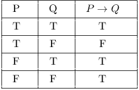 |
| a excludes b | not a or not b |  |

def WALKSAT(clauses, p, max_flips)
  returns:a satisfying model or failure
   inputs: clauses, a set of clauses in propositional logic

           p, the probability of choosing to do a "random walk" move, typically around 0.5

          max_flips, number of flips allowed before giving up
   model ← a random assignment of true/false to the symbols in clauses
   for i = 1 to max_flips do

      if model satisfies clauses then return model
      clause ← a randomly selected clause from clauses that is false in model

       with probability p flip the value in model of a randomly selected symbol from clause

       else flip whichever symbol in clause maximizes the number of satisfied clauses

   return failure
Here's WALKSAT applied to simulated annealing:
def WALKSATsortof(problem,p)
  returns: a solution state
  input: probability p of "local seaarch"
  current ← problem.INITIAL-STATE
  for t = 1 to Tmax do
     next ← copy(curret)
     pick an attribute at random
     if rand() < p then change attrtibute at random
     else search across attribute's range for the value that most improves VALUE(next)
     if next is better than current then current ← next

return currentThis is DODGE1
(Don't go to the "same place" twice.)
(Where "same place" means "within


So lets try that for some text mining, classification tasks

- Control
$N_1=N_2=15,\epsilon=0.2$ - Assign weights w = 0 to configuration options.
- Stagger:
$N_1$ times repeat:- Randomly pick an options, favoring those with most weight;
- Run and reweigh:
- Configure and executing data pre-processors and learners using that option;
- Let
$\Delta$ be min distance ofconfig.scoreto any other score. config.options-- if Delta < .2 else config.options++
- Chop:
$N_2$ time repeat:- Find lowest and highest weight
$a,z$ ever seen so far - Let
$x_i$ be- anything between
$a_i$ and$(a_i ... z_i)/2$ (for numerics) -
$a_i$ (for symbols)
- anything between
- Configure and executing data pre-processors and learners using
$x$ - Run and reweigh
- Find lowest and highest weight
- Return the best option found in the above.
(Please note that this page uses materials from Joel Gruz's excellent book Data Mining from Scratch. Also, if there is anything missing from the following code, please see the raw source code. )

- One thing to note about the following is that is shows an optimizer in the middle of a data miner.
- Another thing to note is that this optimizer makes many assumptions about the kind of function it is exploring.
- The benefit of making those assumptions is that, using those assumptions, certain calculations are fast to compute;
- But if the data does not correspond to those assumptions, then the resulting core fit will be very poor.
- All the above learners do not make these assumptions
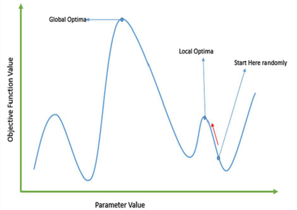
- Gradient descent (gradient ascent) methods can get trapped by local optima . In most real-world situations, we have many peaks and many valleys, which causes such methods to fail, as they suffer from an inherent tendency of getting stuck at the local optima:
def minimize_stochastic(target_fn, gradient_fn, x, y, theta_0, alpha_0=0.01):
    data = list(zip(x, y))
    theta = theta_0                             # initial guess
    alpha = alpha_0                             # initial step size
    min_theta, min_value = None, float("inf")   # the minimum so far
    iterations_with_no_improvement = 0
    # if we ever go 100 iterations with no improvement, stop
    while iterations_with_no_improvement < 100:
        value = sum( target_fn(x_i, y_i, theta) for x_i, y_i in data )
        if value < min_value:
            # if we've found a new minimum, remember it
            # and go back to the original step size
            min_theta, min_value = theta, value
            iterations_with_no_improvement = 0
            alpha = alpha_0
        else:
            # otherwise we're not improving, so try shrinking the step size
            iterations_with_no_improvement += 1
            alpha *= 0.9

        # and take a gradient step for each of the data points
        for x_i, y_i in in_random_order(data):
            gradient_i = gradient_fn(x_i, y_i, theta)
            theta = vector_subtract(theta, scalar_multiply(alpha, gradient_i))
    return min_theta

def squared_error(x_i, y_i, theta):
    alpha, beta = theta
    return error(alpha, beta, x_i, y_i) ** 2

def squared_error_gradient(x_i, y_i, theta):
    alpha, beta = theta
    return [-2 * error(alpha, beta, x_i, y_i),       # alpha partial derivative
            -2 * error(alpha, beta, x_i, y_i) * x_i] # beta partial derivative

def in_random_order(data):
    indexes = [i for i, _ in enumerate(data)]  # create a list of indexes
    random.shuffle(indexes)                    # shuffle them
    for i in indexes:                          # return the data in that order
        yield data[i]

def vector_subtract(v, w):
    return [v_i - w_i for v_i, w_i in zip(v,w)]

def scalar_multiply(c, v):
return [c * v_i for v_i in v]One of the most basic data mining algorithms is least squares regression. This algorithm tries to fit a straight line to a set of points. The best line is the one that reduces the square of the distance between the predicted and actual values.

The above stochastic gradient descent (SDG) method will be used to optimize the β parameters of equations like
y=α+β1x1+β2x2+β3x3+ ...
(and in this case "optimize" means "guess β values in order to reduce the prediction error". SDG is a perfect illustration of how "optimize" and "data mine" and really very tightly connected.
For example:
# here are lots of examples of x1,x2,x3
xs = [[1,49,4,0],[1,41,9,0],[1,40,8,0],[1,25,6,0],[1,21,1,0],[1,21,0,0],[1,19,3,0],
      [1 ,19,0,0],[1,18,9,0],[1,18,8,0],[1,16,4,0],[1,15,3,0],[1,15,0,0],[1,15,2,0],
      [1,15,7,0],[1 ,14,0,0],[1,14,1,0],[1,13,1,0],[1,13,7,0],[1,13,4,0],[1,13,2,0],
      [1,12,5,0],[1,12,0,0],[1,11,9,0],[1,10,9,0],[1,10,1,0],[1,10,1,0],[1,10,7,0],
      [1,10,9,0],[1,10,1,0],[1,10,6,0],[1,10,6,0],[1,10,8,0],[1,10,10,0],[1,10,6,0],
      [1,10,0,0],[1,10,5,0],[1,10,3,0],[1,10,4,0],[1,9,9,0],[1,9,9,0],[1,9,0,0],
      [1,9,0,0],[1,9,6,0],[1,9,10,0],[1,9,8,0],[1,9,5,0],[1,9,2,0],[1,9,9,0],
      [1,9,10,0],[1,9,7,0],[1,9,2,0],[1,9,0,0],[1,9,4,0],[1,9,6,0],[1,9,4,0],
      [1,9,7,0],[1,8,3,0],[1,8,2,0],[1,8,4,0],[1,8,9,0],[1,8,2,0],[1,8,3,0],
      [1,8,5,0],[1,8,8,0],[1,8,0,0],[1,8,9,0],[1,8,10,0],[1,8,5,0],[1,8,5,0],
      [1,7,5,0],[1,7,5,0],[1,7,0,0],[1,7,2,0],[1,7,8,0],[1,7,10,0],[1,7,5,0],
      [1,7,3,0],[1,7,3,0],[1,7,6,0],[1,7,7,0],[1,7,7,0],[1,7,9,0],[1,7,3,0],
      [1,7,8,0],[1,6,4,0],[1,6,6,0],[1,6,4,0],[1,6,9,0],[1,6,0,0],[1,6,1,0],
      [1,6,4,0],[1,6,1,0],[1,6,0,0],[1,6,7,0],[1,6,0,0],[1,6,8,0],[1,6,4,0],
      [1,6,2,1],[1,6,1,1],[1,6,3,1],[1,6,6,1],[1,6,4,1],[1,6,4,1],[1,6,1,1],
      [1,6,3,1],[1,6,4,1],[1,5,1,1],[1,5,9,1],[1,5,4,1],[1,5,6,1],[1,5,4,1],
      [1,5,4,1],[1,5,10,1],[1,5,5,1],[1,5,2,1],[1,5,4,1],[1,5,4,1],[1,5,9,1],
      [1,5,3,1],[1,5,10,1],[1,5,2,1],[1,5,2,1],[1,5,9,1],[1,4,8,1],[1,4,6,1],
      [1,4,0,1],[1,4,10,1],[1,4,5,1],[1,4,10,1],[1,4,9,1],[1,4,1,1],[1,4,4,1],
      [1,4,4,1],[1,4,0,1],[1,4,3,1],[1,4,1,1],[1,4,3,1],[1,4,2,1],[1,4,4,1],
      [1,4,4,1],[1,4,8,1],[1,4,2,1],[1,4,4,1],[1,3,2,1],[1,3,6,1],[1,3,4,1],
      [1,3,7,1],[1,3,4,1],[1,3,1,1],[1,3,10,1],[1,3,3,1],[1,3,4,1],[1,3,7,1],
      [1,3,5,1],[1,3,6,1],[1,3,1,1],[1,3,6,1],[1,3,10,1],[1,3,2,1],[1,3,4,1],
      [1,3,2,1],[1,3,1,1],[1,3,5,1],[1,2,4,1],[1,2,2,1],[1,2,8,1],[1,2,3,1],
      [1,2,1,1],[1,2,9,1],[1,2,10,1],[1,2,9,1],[1,2,4,1],[1,2,5,1],[1,2,0,1],
      [1,2,9,1],[1,2,9,1],[1,2,0,1],[1,2,1,1],[1,2,1,1],[1,2,4,1],[1,1,0,1],
      [1,1,2,1],[1,1,2,1],[1,1,5,1],[1,1,3,1],[1,1,10,1],[1,1,6,1],[1,1,0,1],
      [1,1,8,1],[1,1,6,1],[1,1,4,1],[1,1,9,1],[1,1,9,1],[1,1,4,1],[1,1,2,1],
      [1,1,9,1],[1,1,0,1],[1,1,8,1],[1,1,6,1],[1,1,1,1],[1,1,1,1],[1,1,5,1]
      ]

# each i-th item from "ys" is the output see from the i-th input from "xs"

ys = [68.77, 51.25, 52.08, 38.36, 44.54, 57.13, 51.4, 41.42, 31.22,
34.76, 54.01, 38.79, 47.59, 49.1, 27.66, 41.03, 36.73, 48.65, 28.12,
46.62, 35.57, 32.98, 35, 26.07, 23.77, 39.73, 40.57, 31.65, 31.21,
36.32, 20.45, 21.93, 26.02, 27.34, 23.49, 46.94, 30.5, 33.8, 24.23,
21.4, 27.94, 32.24, 40.57, 25.07, 19.42, 22.39, 18.42, 46.96, 23.72,
26.41, 26.97, 36.76, 40.32, 35.02, 29.47, 30.2, 31, 38.11, 38.18,
36.31, 21.03, 30.86, 36.07, 28.66, 29.08, 37.28, 15.28, 24.17,
22.31, 30.17, 25.53, 19.85, 35.37, 44.6, 17.23, 13.47, 26.33, 35.02,
32.09, 24.81, 19.33, 28.77, 24.26, 31.98, 25.73, 24.86, 16.28,
34.51, 15.23, 39.72, 40.8, 26.06, 35.76, 34.76, 16.13, 44.04, 18.03,
19.65, 32.62, 35.59, 39.43, 14.18, 35.24, 40.13, 41.82, 35.45,
36.07, 43.67, 24.61, 20.9, 21.9, 18.79, 27.61, 27.21, 26.61, 29.77,
20.59, 27.53, 13.82, 33.2, 25, 33.1, 36.65, 18.63, 14.87, 22.2,
36.81, 25.53, 24.62, 26.25, 18.21, 28.08, 19.42, 29.79, 32.8, 35.99,
28.32, 27.79, 35.88, 29.06, 36.28, 14.1, 36.63, 37.49, 26.9, 18.58,
38.48, 24.48, 18.95, 33.55, 14.24, 29.04, 32.51, 25.63, 22.22, 19,
32.73, 15.16, 13.9, 27.2, 32.01, 29.27, 33, 13.74, 20.42, 27.32,
18.23, 35.35, 28.48, 9.08, 24.62, 20.12, 35.26, 19.92, 31.02, 16.49,
12.16, 30.7, 31.22, 34.65, 13.13, 27.51, 33.2, 31.57, 14.1, 33.42,
17.44, 10.12, 24.42, 9.82, 23.39, 30.93, 15.03, 21.67, 31.09, 33.29,
22.61, 26.89, 23.48, 8.38, 27.81, 32.35, 23.84]

random.seed(0)
beta= estimate_beta(xs,ys)
print(beta)
This prints
- [30.619881701311712, 0.9702056472470465, -1.8671913880379478, 0.9163711597955347]
- i.e. y= 30.62 + 0.97x1 - 1.87x2 + 0.92x3
All the above is surprisingly easy to code, given access to SGD.
To handle this, we need a vector for
the xs values and the
βs :
- [ α, β1x1, β2x2, β3x3,... ]
which we can use in the following functions to find predictions, errors, and squared errors (in a manner similar to the above).
def dot(v, w)                     : return sum(v_i * w_i for v_i, w_i in zip(v, w))
def predicts(x_i, beta)           : return dot(x_i, beta)
def errors(x_i, y_i, beta)        : return y_i - predicts(x_i, beta)
def squared_errors(x_i, y_i, beta): return errors(x_i, y_i, beta) ** 2
Then we do some gradient descent. This is like sking, when you are drunk. In this approach, to get to the bottom of a hill:
- Stand anywhere
- Lean over to every other point and write down the slope between you and them
- Move yourself along the average slope.
def estimate_beta(x, y):
    beta_initial = [random.random() for x_i in x[0]]
    return minimize_stochastic(squared_errors,
                               squared_error_gradients,
                               x, y,
                               beta_initial,
                               0.001)

def squared_error_gradients(x_i, y_i, beta):
    """the gradient corresponding to the ith squared error term.
       Derived via calculus applied to squared_errors."""
    return [-2 * x_ij * errors(x_i, y_i, beta)
            for x_ij in x_i]
Footnotes
-
Amritanshu Agrawal, Xueqi Yang, Rishabh Agrawal, Rahul Yedida, Xipeng Shen, and Tim Menzies. 2022. Simpler Hyperparameter Optimization for Software Analytics: Why, How, When? IEEE Trans. Softw. Eng. 48, 8 (Aug. 2022), 2939–2954. https://doi.org/10.1109/TSE.2021.3073242 ↩