The SIFT User's Guide
Out of Date: This guide was written for SIFT 1.x and does not properly describe the newer SIFT 2.x application.
The Satellite Information Familiarization Tool (SIFT) was designed at SSEC/CIMSS to support scientists during forecaster training events. It provides a graphical interface for visualization and basic analysis of geostationary satellite data.
The first thing to do with SIFT: Download the version you wish to use. The latest downloads are available at this ftp site. There are versions for unix (.gz), Apple (.dmg) and Windows (.exe); Grab what you need, and download and expand it. You do not need to compile anything.
SIFT will directly read in GOES-16 (and GOES-17) data that has been requested and received from the NOAA CLASS Archive. Many different data sources are available from CLASS: You want to choose 'GOES-R Series ABI Products (GRABIPRD) (partially restricted L1b and L2+ Data Products)' and then click on the 'GO' next to the ">>" that sits next to the drop down menu that includes all the products. SIFT will display either Radiance/Reflectance files, or CMI (Cloud/Moisture Imagery) files. Order what you want, and await the email from CLASS that says it is ready to be downloaded. Download the data onto your computer.
Once the data are in place, start up SIFT. How this is done varies by operating system. In RedHat linux, for example, it's done by executing a script. On Windows 10, you might click on an Icon. The SIFT Window should appear, as shown below.(Version 1.0.3 is being used).
The image above shows SIFT. In addition to the main SIFT display, note other windows that -- upon opening -- are not populated with information (Yet): The 'Layers' window (upper right); the 'Area Probe Graphs' (upper right, underneath the 'Layers' window; you can bring it forward by clicking the tab); the 'Layer Details' window (center right); and 'Composite Details' that are in the lower right: 'Layer Details' ; 'RGB Bounds'; 'Timeline')
When you have data, under the 'File' Tab in the SIFT window, click on 'Open File Wizard' -- or Ctrl-O -- that will require you to specify the reader for the data being loaded (for example, GOES-R ABI Level 1b; Himawari AHI Level 1b (HSD), etc). Then you will choose the files stored on your computer to be loaded. (In versions 1.0.6 and earlier, File-Open (CTRL-O) under the 'File' Tab will lead you directly to a dialog where you select the SIFT-readable netCDF files on your computer). If you’ve previously downloaded the data, you can also ‘Open from Cache’ or ‘Open Recent’. SIFT also allows you to open Himawari imagery -- but you have to configure the data to something resembling the GOES-R files first, using AXI-tools that are available at SSEC/CIMSS.
(Here's a Video on Youtube that shows data being loaded -- using SIFT Version 1.1.3 -- and also shows how to change the color enhancement)
When data have been loaded, the ‘Layers’ and ‘Layer Details’ windows within the SIFT display will contain information. In the example below, all 16 ABI channels from 15:07:19 on November 2017 have been loaded. Note that Band 1 is highlighted – in blue – in the ‘Layers’ list – this means it’s being displayed. The check marks in the other bands means they are ready to be displayed if you animate this field (in which case you’ll see all 16 bands sequentially) or if you hit the ‘Pg Up’ key (Up Arrow) or ‘Pg Dn’ key (Down Arrow) on the keyboard to cycle through the bands. (If you load multiple times, the Right/Left arrows change view of the scene to the next/previous time, respectively). If the Check Box is checked, then the top-most check-box will be what you see on the screen. When SIFT animates, you’ll note that check boxes are turned off. You can also turn them off manually by clicking on them, toggling them off.

In this example above, all 16 ABI Bands for one time, for the CONUS scan sector, have been loaded. The projection used to display is LCC CONUS -- that can be changed by clicking on the drop-down menu and choosing a different pre-loaded projection (For example, GOES-East, a full-disk representation centered at 75.2 degrees W Longitude). Loading the data forces changes in the SIFT display window also, as you can see above. The 'Layers' window has information in it, and the 'Layer Details' window is also filled. If you right-click on the SIFT display, you will activate the 'probe' feature as shown below. That Red Dot shows where the Probe is, and values for all loaded bands are displayed.
If you want to expand the Layer Probe window, that is doable: double click on the top of the window and drag it out, and reposition is as shown below. A good lab exercise for students is to have them view the probe values in isolation and intuit the scene that must be being sensed. For the example below, obvious questions might be (1) Why does Band 4 have such low reflectance values? (2) Why are Band 7 brightness temperatures so warm?
The animation at this link (Link) steps through all 16 bands. The probe has been moved to a different location than shown above.

In the image above, the Layer List has been popped back into (reattached to) the SIFT window -- this is done by double-clicking on the title bar. Note that the cursor is clicking on the 'Region' tab. Do this to create a sub-region for which you want to investigate satellite band properties. After clicking, define a polygon by right-clicking on locations. Close the polygon by right-clicking on the initial point. This sequence of events is shown in this animation (Link).
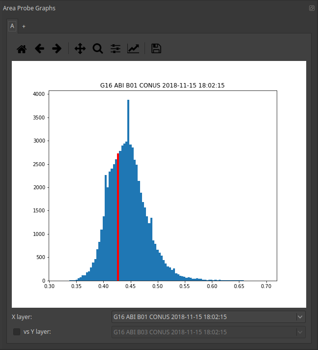
When you have defined a region, the 'Area Probe Graphs' window on the right-hand side of the main SIFT display becomes active (this window shares space with the 'Layers' window; if you click on 'Area Probe Graphs' the window will be brought to the forefront, as shown below).
You can also Double Click on the title bar of the Area Probe Graphs window and separate it from the SIFT Display, and enlarge it, as shown below. Note the choices available at the bottom -- the bar graph shows Band 1 -- but any band that is displayed can also be shown in bar graph form for the region selected. And you can compare bands as well by clicking on the 'VS' box, and choosing the second band.
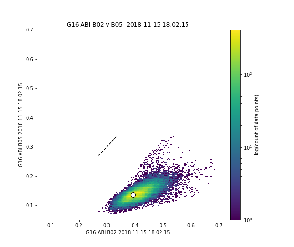
The image below shows Band 2 vs. Band 5 (that is, visible vs. snow-ice band). The labels have been modified from their default values, shown in the bar graph above, and the axes have been defined. The dashed line shows x = y. In this case, Band 2 reflectances are much greater than Band 5 reflectances, a characteristic feature of ice clouds.
There are a couple of YouTube tutorials available. A shorter video describes how to use SIFT to create the Split Window Difference that can be used to detect dust (or moisture differences) in the atmosphere. (Link). A second video describes how to create an Air Mass RGB. (Link).