written by Junvie Pailden
# install the necessary packages if it doesn't exist
if (!require(mosaic)) install.packages(`mosaic`)
if (!require(dplyr)) install.packages(`dplyr`)
# load the packages
library(mosaic)
library(dplyr)The data below presents data on the first 18 young climbers whose parents consented to participate in an experiment on the effects of acute mountain sickness (AMS).
# one method to enter small data sets directly using `data.frame()`
AMS.dat <- data.frame(
  gender = c("male", "female", "male", "male", "male", "male",
              "female", "female", "male", "female", "female", "male",
              "female", "female", "male", "female", "female", "male"),
  age = c(12.90, 13.34, 12.39, 13.95, 13.63, 13.62, 12.55, 13.54, 12.34,
           13.74, 13.78, 14.05, 14.22, 13.91, 14.39, 13.54, 13.85, 14.11)
)
AMS.dat # print the entire data frame
#    gender  age
# 1    male 12.9
# 2  female 13.3
# 3    male 12.4
# 4    male 13.9
# 5    male 13.6
# 6    male 13.6
# 7  female 12.6
# 8  female 13.5
# 9    male 12.3
# 10 female 13.7
# 11 female 13.8
# 12   male 14.1
# 13 female 14.2
# 14 female 13.9
# 15   male 14.4
# 16 female 13.5
# 17 female 13.8
# 18   male 14.1
An experimental plan is to assign the participants into two treatments by flipping a coin until the first treatment has been assign nine times; then assign the second treatment to the remaining subjects.
We can randomly select nine subjects to the first treatment using the function sample_n() from the package dplyr. sample_n() randomly select n rows from a data frame.
# randomly select `size = 9` subjects to treatment 1
trt1 <- sample_n( AMS.dat, size = 9)
trt1
#    gender  age
# 5    male 13.6
# 10 female 13.7
# 3    male 12.4
# 4    male 13.9
# 1    male 12.9
# 12   male 14.1
# 17 female 13.8
# 15   male 14.4
# 6    male 13.6
If we want to randomly select, instead, 4 males and 5 females separately (this is called blocking in experiments), we do the following
-
use
filter()to assign the male and female subjects to separate data frames, -
use
sample_n()to randomly select the subjects.
AMS.male <- filter(AMS.dat, gender == "male")
# use boolean argument `gender == male` to select male subjects only
AMS.male
#   gender  age
# 1   male 12.9
# 2   male 12.4
# 3   male 13.9
# 4   male 13.6
# 5   male 13.6
# 6   male 12.3
# 7   male 14.1
# 8   male 14.4
# 9   male 14.1
AMS.female <- filter(AMS.dat, gender == "female")
# use boolean argument `gender == female` to select male subjects only
AMS.female
#   gender  age
# 1 female 13.3
# 2 female 12.6
# 3 female 13.5
# 4 female 13.7
# 5 female 13.8
# 6 female 14.2
# 7 female 13.9
# 8 female 13.5
# 9 female 13.8
trt1.male <- sample_n( AMS.male, size = 4) # randomly select 4 male subjects
trt1.male
#   gender  age
# 9   male 14.1
# 4   male 13.6
# 7   male 14.1
# 3   male 13.9
trt1.female <- sample_n( AMS.female, size = 5) # randomly select 5 female subjects
trt1.female
#   gender  age
# 5 female 13.8
# 9 female 13.8
# 3 female 13.5
# 4 female 13.7
# 7 female 13.9The data mtcars was extracted from the 1974 Motor Trend US magazine, and comprises fuel consumption and 10 aspects of automobile design and performance for 32 automobiles (1973–74 models). Check the helpfile by typing ?mtcars in the console for more details regarding the data.
str(mtcars) # structure
# 'data.frame': 32 obs. of  11 variables:
#  $ mpg : num  21 21 22.8 21.4 18.7 18.1 14.3 24.4 22.8 19.2 ...
#  $ cyl : num  6 6 4 6 8 6 8 4 4 6 ...
#  $ disp: num  160 160 108 258 360 ...
#  $ hp  : num  110 110 93 110 175 105 245 62 95 123 ...
#  $ drat: num  3.9 3.9 3.85 3.08 3.15 2.76 3.21 3.69 3.92 3.92 ...
#  $ wt  : num  2.62 2.88 2.32 3.21 3.44 ...
#  $ qsec: num  16.5 17 18.6 19.4 17 ...
#  $ vs  : num  0 0 1 1 0 1 0 1 1 1 ...
#  $ am  : num  1 1 1 0 0 0 0 0 0 0 ...
#  $ gear: num  4 4 4 3 3 3 3 4 4 4 ...
#  $ carb: num  4 4 1 1 2 1 4 2 2 4 ...
In the package dplyr we can use the following functions to select random rows from the data frame.
- use
sample_n()to randomly select fixed number of rows.
# Sample fixed number per group
sample_n(mtcars, 10)  # randomly select 10 rows
#                      mpg cyl  disp  hp drat   wt qsec vs am gear carb
# Fiat 128            32.4   4  78.7  66 4.08 2.20 19.5  1  1    4    1
# Pontiac Firebird    19.2   8 400.0 175 3.08 3.85 17.1  0  0    3    2
# Chrysler Imperial   14.7   8 440.0 230 3.23 5.34 17.4  0  0    3    4
# Merc 280            19.2   6 167.6 123 3.92 3.44 18.3  1  0    4    4
# Lincoln Continental 10.4   8 460.0 215 3.00 5.42 17.8  0  0    3    4
# Merc 450SL          17.3   8 275.8 180 3.07 3.73 17.6  0  0    3    3
# Lotus Europa        30.4   4  95.1 113 3.77 1.51 16.9  1  1    5    2
# Mazda RX4           21.0   6 160.0 110 3.90 2.62 16.5  0  1    4    4
# Cadillac Fleetwood  10.4   8 472.0 205 2.93 5.25 18.0  0  0    3    4
# Merc 450SLC         15.2   8 275.8 180 3.07 3.78 18.0  0  0    3    3
sample_n(mtcars, 10, replace = TRUE) # randomly select 10 rows with replacement
#                      mpg cyl  disp  hp drat   wt qsec vs am gear carb
# Hornet 4 Drive      21.4   6 258.0 110 3.08 3.21 19.4  1  0    3    1
# Mazda RX4           21.0   6 160.0 110 3.90 2.62 16.5  0  1    4    4
# Lincoln Continental 10.4   8 460.0 215 3.00 5.42 17.8  0  0    3    4
# Toyota Corona       21.5   4 120.1  97 3.70 2.46 20.0  1  0    3    1
# Hornet 4 Drive.1    21.4   6 258.0 110 3.08 3.21 19.4  1  0    3    1
# Toyota Corolla      33.9   4  71.1  65 4.22 1.83 19.9  1  1    4    1
# Datsun 710          22.8   4 108.0  93 3.85 2.32 18.6  1  1    4    1
# Toyota Corolla.1    33.9   4  71.1  65 4.22 1.83 19.9  1  1    4    1
# Volvo 142E          21.4   4 121.0 109 4.11 2.78 18.6  1  1    4    2
# Ferrari Dino        19.7   6 145.0 175 3.62 2.77 15.5  0  1    5    6
We can also randomly select rows from the data with selection probabilities proportional to a given set or variable.
# select 10 rows with prob'y proportional to mpg size,
# i.e., higher mpg cars will likely be more selected
sample_n(mtcars, 10, weight = mpg)
#                     mpg cyl disp  hp drat   wt qsec vs am gear carb
# Merc 230           22.8   4  141  95 3.92 3.15 22.9  1  0    4    2
# Volvo 142E         21.4   4  121 109 4.11 2.78 18.6  1  1    4    2
# Cadillac Fleetwood 10.4   8  472 205 2.93 5.25 18.0  0  0    3    4
# Ferrari Dino       19.7   6  145 175 3.62 2.77 15.5  0  1    5    6
# Porsche 914-2      26.0   4  120  91 4.43 2.14 16.7  0  1    5    2
# Maserati Bora      15.0   8  301 335 3.54 3.57 14.6  0  1    5    8
# AMC Javelin        15.2   8  304 150 3.15 3.44 17.3  0  0    3    2
# Merc 450SL         17.3   8  276 180 3.07 3.73 17.6  0  0    3    3
# Toyota Corona      21.5   4  120  97 3.70 2.46 20.0  1  0    3    1
# Chrysler Imperial 14.7 8 440 230 3.23 5.34 17.4 0 0 3 4- use
sample_frac()to sample fixed fraction per group
# sample_frac(mtcars) # default, randomly re-arrange all rows
sample_frac(mtcars, 0.1) # randomly select 10% of the rows
#                    mpg cyl disp  hp drat   wt qsec vs am gear carb
# Chrysler Imperial 14.7   8  440 230 3.23 5.34 17.4  0  0    3    4
# Datsun 710        22.8   4  108  93 3.85 2.32 18.6  1  1    4    1
# Dodge Challenger  15.5   8  318 150 2.76 3.52 16.9  0  0    3    2
sample_frac(mtcars, 0.2) # randomly select 20% of the rows
#                      mpg cyl  disp  hp drat   wt qsec vs am gear carb
# Toyota Corolla      33.9   4  71.1  65 4.22 1.83 19.9  1  1    4    1
# Fiat X1-9           27.3   4  79.0  66 4.08 1.94 18.9  1  1    4    1
# Porsche 914-2       26.0   4 120.3  91 4.43 2.14 16.7  0  1    5    2
# Merc 450SL          17.3   8 275.8 180 3.07 3.73 17.6  0  0    3    3
# Lincoln Continental 10.4   8 460.0 215 3.00 5.42 17.8  0  0    3    4
# Merc 280 19.2 6 167.6 123 3.92 3.44 18.3 1 0 4 4Simulating a random sample is straightforward in R.
sample(x, size, replace = FALSE, prob = NULL)
takes a sample of the specified size from the elements of x by sampling either with or without replacement. To sample with replacement, type replace=TRUE. To sample without replacement, enter replace=FALSE.
Simulate 1,000 rolls of a fair die and determine the frequency of occurrence of each possible outcome. We do not need to provide the argument prob since we assume that each outcome of tossing a die is equally likely.
dice <- 1:6 # store possible outcomes as vector
rolls <- sample(x = dice,
                size = 1000, # number of rolls
                replace = TRUE) # selecting with replacement
tally(rolls) # tally the results
# X
#   1   2   3   4   5   6
# 163 161 166 147 184 179
tally(rolls)/1000  # proportion of outcomes, 1/6 for each
# X
#     1     2     3     4     5     6
# 0.163 0.161 0.166 0.147 0.184 0.179
The sampling need not be uniform or equally likely. Probabilities of selecting the values in x can be specified with the argument prob.
For example, suppose we want to simulate 100 tosses of a biased coin with probabilities Pr(Head) = 0.60 and Pr(Tail) = 0.40.
coin <- c("Head", "Tail") # possible outcome
coin.toss <- sample(coin,
               prob = c(0.6, 0.4),
               size = 100,
               replace = TRUE)
tally(coin.toss) # tally the results
# X
# Head Tail
#   46   54
We can repeat this sampling generating different results.
tally( sample(coin,
               prob = c(0.6, 0.4),
               size = 100,
               replace = TRUE))
# X
# Head Tail
#   60   40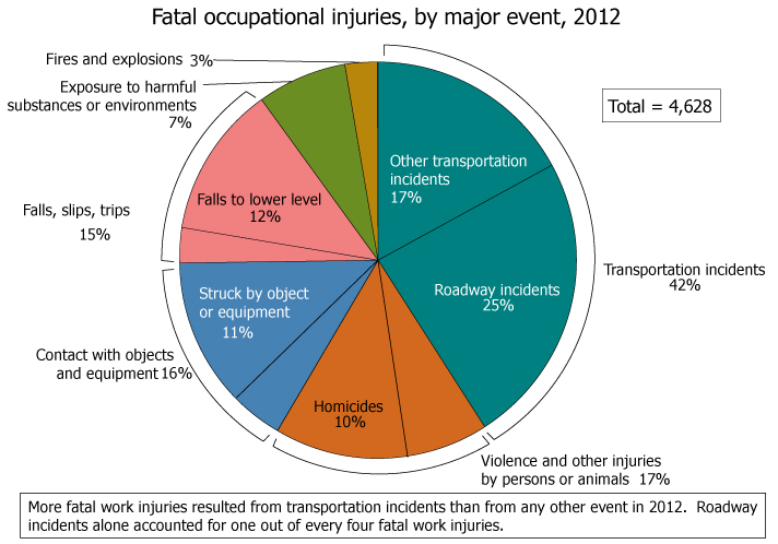
The pie chart above was lifted from an article in riskandinsruance.com.
Suppose a large insurance company wanted to model the next 500 fatal workplace accident claims. We can run an experiment to generate one possible realization.
event.accident <- c("transpo", "violence", "contact", "falls", "exposure", "fires") # set type of accident categories
p.accident <- c(0.42, 0.17, 0.16, 0.15, 0.07, 0.03) # set prob'ys
sum(p.accident) # verify
# [1] 1
s.work <- sample(event.accident,
                 prob = p.accident,
                 size = 500,
                 replace = TRUE)
tally(s.work) # count of type of accident
# X
#  contact exposure    falls    fires  transpo violence
#       79       32       72       17      218       82
tally(s.work)/500 # convert to proportions
# X
#  contact exposure    falls    fires  transpo violence
#    0.158    0.064    0.144    0.034    0.436    0.164
If we run the same experiment again, we might not get the same outcomes.
tally(sample(event.accident,
                 prob = p.accident,
                 size = 500,
                 replace = TRUE))
# X
#  contact exposure    falls    fires  transpo violence
#       82       31       68       17      228       74